Table of Birds

Introduction

Birders love birds for their beautiful features, lovely behaviors, and melodious songs. However, there is more to birds than meets the eye. Birds are a diverse group of animals with a wide range of life history traits, habitats, and diets. Some birds are at risk of extinction due to habitat loss, climate change, and other human activities. This table of birds aims to provide a comprehensive overview of bird species around the world, including their life history traits, conservation status, bird call, breeding bird survey data, diet, habitat, range, and similar species.

Link to the final table

Read in data

# load packages 
library(tidyverse)
library(here)
library(janitor)
library(readxl)

Life history, IUCN, bird call, and breeding bird survey

• Life history data

Life history data was collected from a life history database published in Ecology in 2015 by Myhrvold et al. The data contains about 30 life history traits such as body mass, body length, maturity days, longevity, and clutch sizes for 11,548 species of birds, mammals, and reptiles. The data was downloaded from Wiley archive.

• IUCN Red List data

The IUCN’s Red List, short for the International Union for Conservation of Nature’s Red List, is one of the world’s most comprehensive assessments on global extinction risk status for animal, fungus, and plants. Species are ranked in seven categories: Least Concern, Near Threatened, Vulnerable, Endangered, Critically Endangered, Extinct in the Wild, and Extinct. The Red List helps us understand which species are at risk of extinction and what conservation actions are needed to prevent it. The IUCN data was downloaded from GBIF.

• Bird call

Bird call data was collected from Xeno-canto, a website dedicated to sharing wildlife sounds from all over the world. The data was downloaded from GBIF. The data contains 730,958 occurrences of bird calls from 24,931 species around the world. While I only kept audio data, it also contains latitude and longitude of the observation, and the spectrogram of the sound recording.

To keep the data preparation part short, I migrated all the steps of reading, cleaning, exploring, and joining these data in prep_life_history_IUCN_bbs_birdcall.R. Here we simply read in the intermediate data, ready for use.

birds_life_history_IUCN_bbs_birdcall = read_csv(
  here::here(
    "data",
    "intermediate_data",
    "birds_life_history_IUCN_bbs_birdcall.csv"
  )
) 

Take a quick glimpse at the data:

glimpse(birds_life_history_IUCN_bbs_birdcall)

Rows: 75
Columns: 16
$ iucn_red_list              <chr> "Least Concern", "Least Concern", "Least Co…
$ common_name                <chr> "Mute Swan", "Tufted Duck", "Gadwall", "Tun…
$ genus                      <chr> "Cygnus", "Aythya", "Anas", "Cygnus", "Pavo…
$ species                    <chr> "olor", "fuligula", "strepera", "columbianu…
$ scientific_name            <chr> "Cygnus olor", "Aythya fuligula", "Anas str…
$ birth_or_hatching_weight_g <dbl> 221.50, 34.10, 34.05, 181.25, 120.00, 81.80…
$ adult_body_mass_g          <dbl> 10230.00, 701.50, 850.00, 6350.00, 4093.75,…
$ litter_or_clutch_size_n    <dbl> 5.950000, 9.600000, 10.000000, 4.000000, 5.…
$ litters_or_clutches_per_y  <dbl> 1.00, 1.00, 1.00, 1.00, 1.00, 1.00, 2.00, 1…
$ fledging_age_d             <dbl> 135.00, 47.50, 49.50, 60.25, 14.00, 55.00, …
$ male_maturity_d            <dbl> 1095.00, 365.00, 240.00, 730.00, 730.25, 36…
$ female_maturity_d          <dbl> 1183.569, 365.000, 240.000, 1001.069, 730.0…
$ maximum_longevity_y        <dbl> 70.00000, 45.25000, 28.00000, 24.10000, 25.…
$ adult_svl_cm               <dbl> 142.50, 43.50, 52.00, 135.00, 95.00, 77.50,…
$ aou                        <chr> "01782", "01491", "01350", "01800", "03095"…
$ identifier                 <chr> "https://xeno-canto.org/sounds/uploaded/THH…

Note that column aou is the foreign key linking to the USGS breeding bird survey data we will cover below. Column identifier is the URL of bird call media.

USGS breeding bird survey data

USGS Breeding Bird Survey (BBS) project measures bird populations in North America each year. Data of more than 500 species was collected by citizen scientists in U.S., Canada, and Mexico by conducting bird counts along BBS routes throughout the continent.

Data cleaning and transformation steps were also done in prep_life_history_IUCN_bbs_birdcall.R. I summarized annual number of observations for each species to visualize how populations have been changed over time. I also filtered the year of observation to be after 2000 to avoid the situation where species had low number of observations because of incomplete sampling.

annual_num_observation = read_csv(here::here("data", "intermediate_data", "annual_num_observation.csv"))

# This plot shows what the data is about: annual number of observations by species
annual_num_observation |>
  filter(aou == "01320") |> # select a species to show: Mallard
  ggplot() +
  geom_line(aes(x = year, 
                y = num_observation)) +
  theme_bw() +
  labs(title = "Annual Number of Observations of Birds in North America",
       subtitle = "Example species: Mallard",
       x = "Year",
       y = "Number of Observations")

I plan to display the trend of annual number of observations in the final table using sparklines, an in cell trend line of a list of values. To do that, I prepared the number of observation data in a list by species.

# convert the annual number of observation to a list by aou to be used in the table
annual_num_observation_ls = annual_num_observation |>
  summarize(num_observation_trend = list(num_observation),
            .by = aou)

annual_num_observation_ls |> head()

# A tibble: 6 × 2
  aou   num_observation_trend
  <chr> <list>               
1 01320 <dbl [22]>           
2 01330 <dbl [22]>           
3 01340 <dbl [22]>           
4 01350 <dbl [22]>           
5 01360 <dbl [6]>            
6 01370 <dbl [22]>           

Diet

Diet data was download from R package {aviandietdb}. It contains prey data of 759 bird species, along with functions to help summarize data at different taxonomic levels. The complete process of creating the intermediate data of diet is also available in prep_life_history_IUCN_bbs_birdcall.R.

diet = read_csv(here::here("data", "intermediate_data", 'birds_diet_short.csv'))

# add emoji to each category
diet_emoji = diet |>
  mutate(
    emoji = case_when(
      diet == "mammal" ~ "🐀",
      diet == "amphibian" ~ "🐸",
      diet == "bird" ~ "🐦",
      diet == "reptile" ~ "🦎",
      diet == "fish" ~ "🐟",
      diet == "crustacean" ~ "🦀",
      diet == "spider" ~ "🕷",
      diet == "insect" ~ "🪲",
      diet == "plant" ~ "🌿",
      diet == "snail" ~ "🐌",
      diet == "cyanobacteria" ~ "🦠",
      diet == "worm" ~ "🪱",
      diet == "centipede" ~ "🐛",
      diet == "millipede" ~ "🐛",
      diet == "conifer" ~ "🌲",
      diet == "moss" ~ "🌿",
      diet == "fern" ~ "🌿",
      diet == "scallop" ~ "🐚"
    )
  ) 

glimpse(diet_emoji)

Rows: 168
Columns: 3
$ common_name <chr> "Pink-footed Goose", "Greater White-fronted Goose", "Garga…
$ diet        <chr> "plant", "plant", "plant", "snail", "plant", "cyanobacteri…
$ emoji       <chr> "🌿", "🌿", "🌿", "🐌", "🌿", "🦠", "🪲", "🕷", "🌿", "🪲",…

Habitat, photos, and similar species

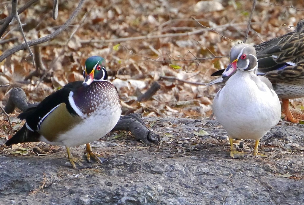
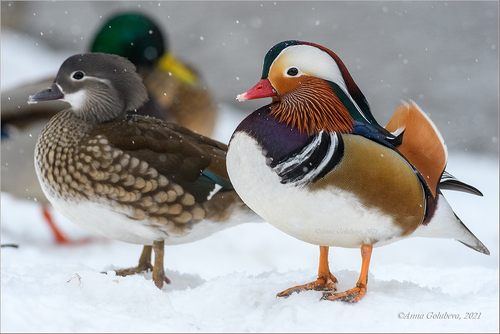
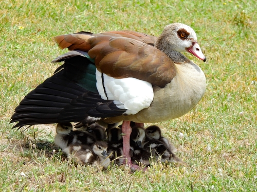
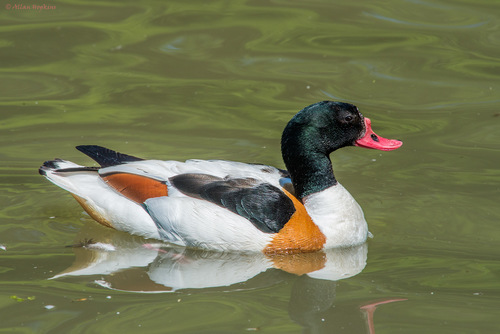
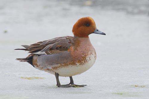
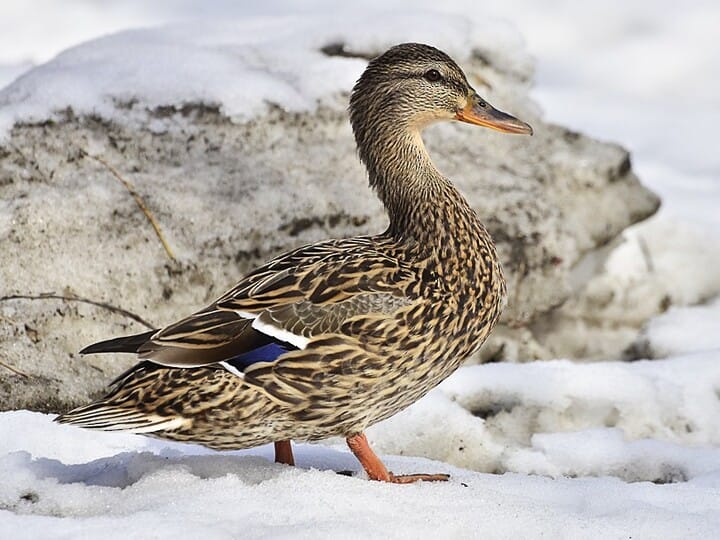
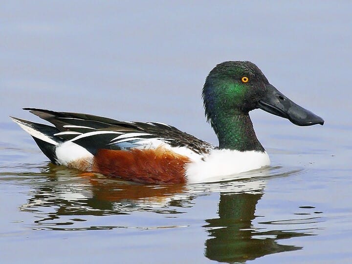
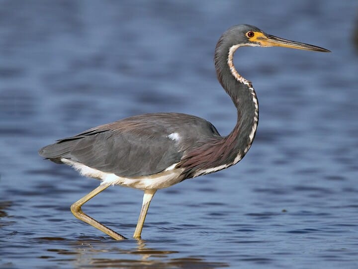
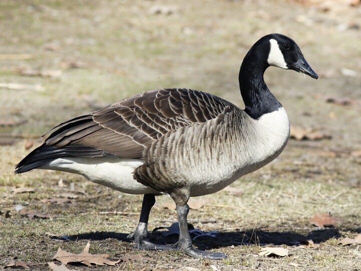
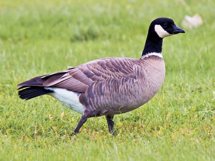
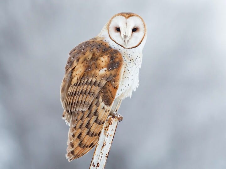
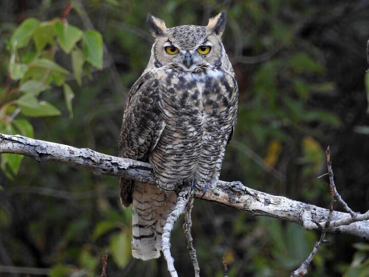
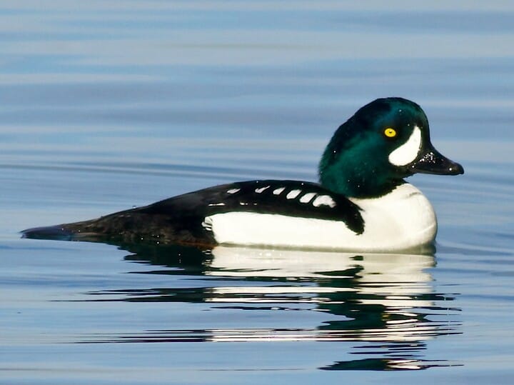
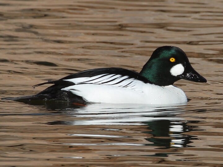
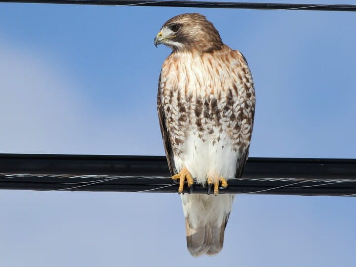
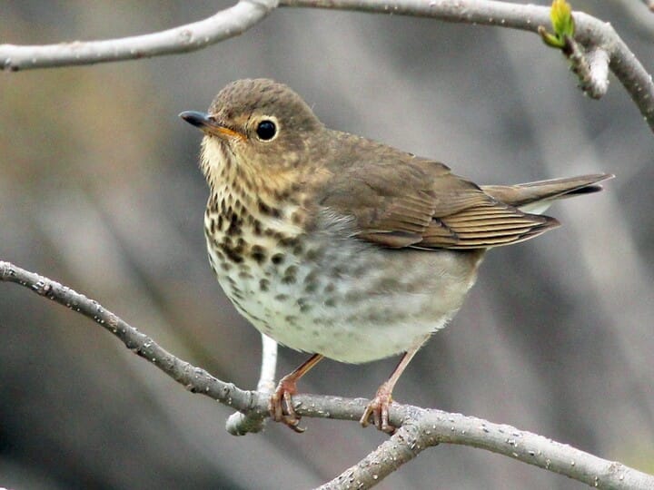
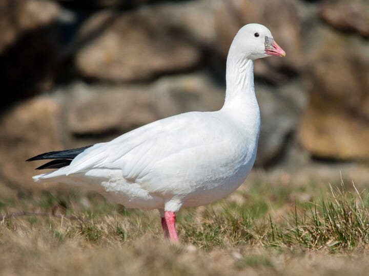
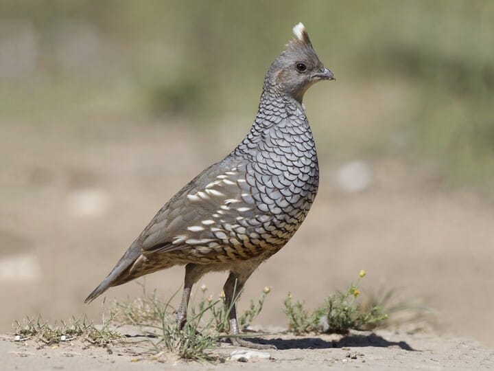
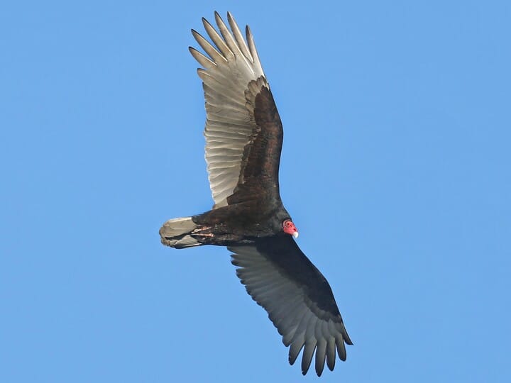
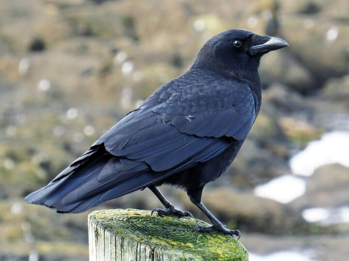
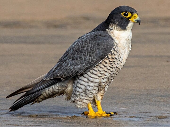
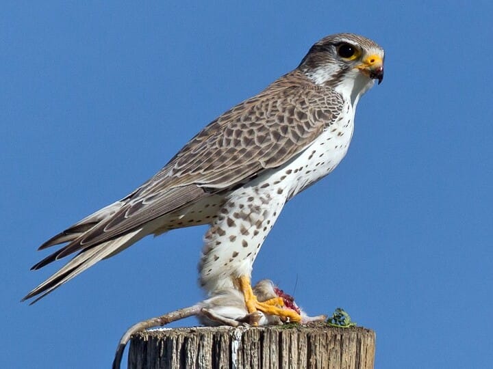
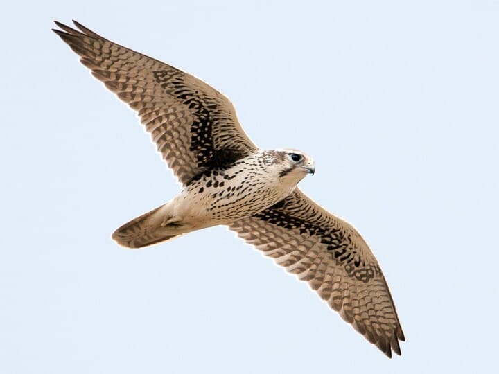
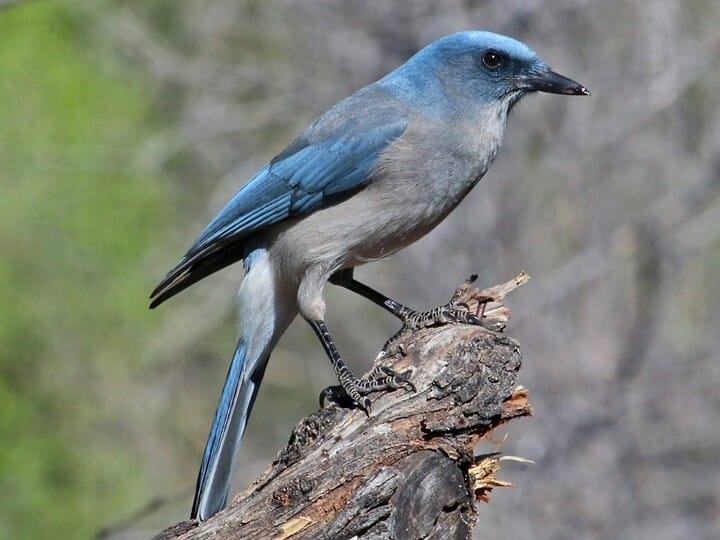
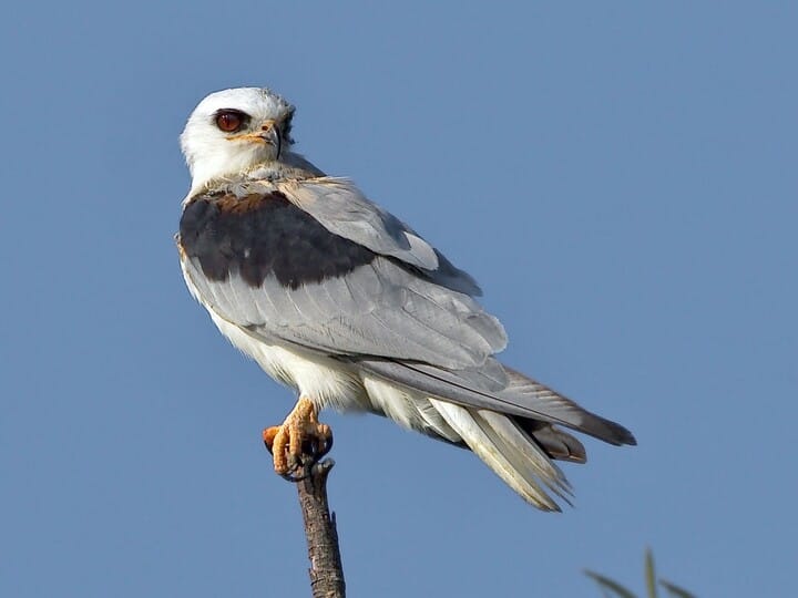
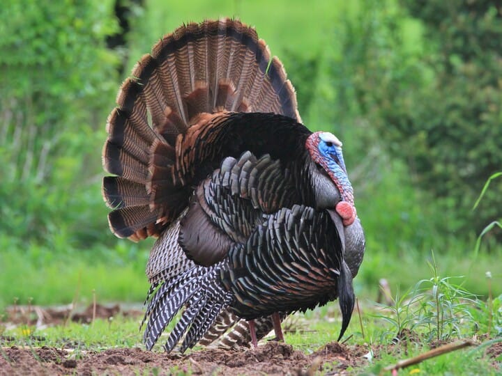
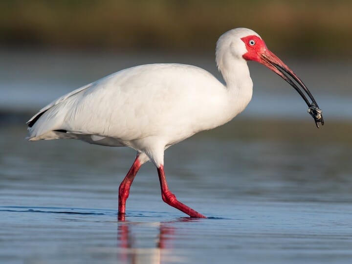
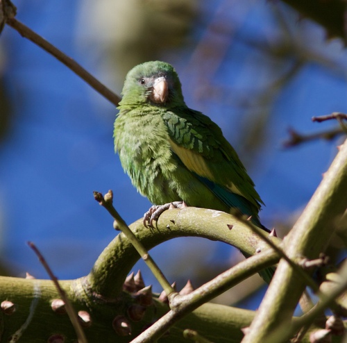
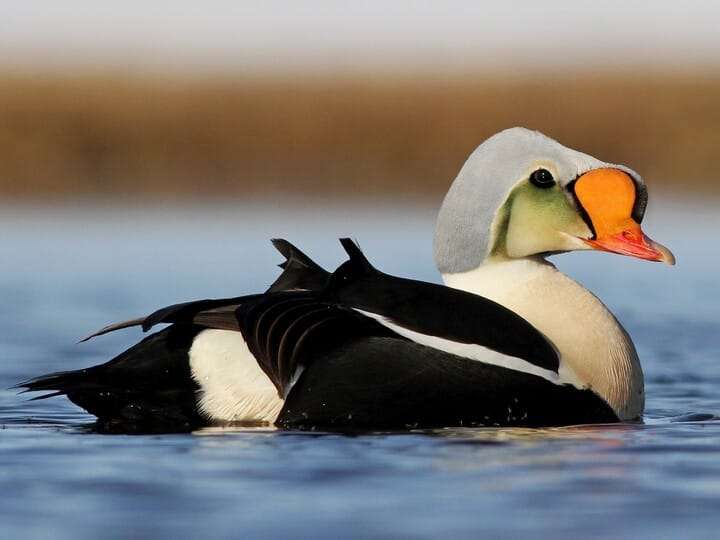
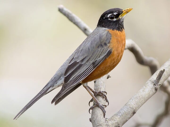
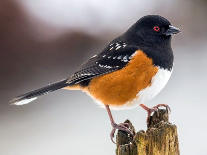
Birds habitat data was collected manually from Animal Biodiversity Web and All About Birds because it was really difficult to find a data source that closely meets my needs. I also manually selected representative and appealing images of the birds and their similar species. Appealing bird photos and external links to similar species are collected from iNaturalist and All About Birds.

# Bird image, similar species and habitat 
birds_sheets = excel_sheets(here("data", "birds.xlsx"))
my_birds = lapply(birds_sheets, function(x){
  read_excel(here("data", "birds.xlsx"), sheet = x) |>
    clean_names()
}) |>
  `names<-`(birds_sheets)

# bird_manual table in my_birds contains birds common name, genus, species along with url to birds images, similar species images, and similar species information
glimpse(my_birds$bird_manual)

Rows: 75
Columns: 7
$ common_name           <chr> "Mute Swan", "Tufted Duck", "Gadwall", "Tundra S…
$ genus                 <chr> "Cygnus", "Aythya", "Anas", "Cygnus", "Pavo", "C…
$ species               <chr> "olor", "fuligula", "strepera", "columbianus", "…
$ image                 <chr> "https://www.allaboutbirds.org/guide/assets/phot…
$ similar_species       <chr> "Tundra Swan", "Greater Scaup", "Green-winged Te…
$ similar_species_image <chr> "https://www.allaboutbirds.org/guide/assets/phot…
$ similar_species_link  <chr> "https://www.allaboutbirds.org/guide/Mute_Swan/s…

# Habitat data with emoji
habitat_emoji = my_birds$habitat |>
  pivot_longer(habitat_1:habitat_8, 
               values_to = "habitat",
               values_drop_na = TRUE) |>
  select(-name) |>
  select(-genus, -species) |>
  # full list of emoji: https://unicode.org/emoji/charts/full-emoji-list.html
  # Use emoji habitat data 
  mutate(emoji = case_when(
    habitat == "desert" ~ "🏜",
    habitat == "agricultural" ~ "🌾",
    habitat == "forest" ~ "🌲",
    habitat == "grassland" ~ "🌿",
    habitat == "coastal" ~  "🏖",
    habitat == "urban" ~ "🏙",
    habitat == "suburban" ~ "🏙",
    habitat == "lakes and ponds" ~ "🌊",
    habitat == "rivers and streams" ~ "🌊",
    habitat == "marsh" ~ "🌊",
    habitat == "estuarine" ~ "🌊",
    habitat == "tundra" ~ "🏔",
    habitat == "taiga" ~ "🌲",
    habitat == "rainforest" ~ "🌳",
    habitat == "mountains" ~ "⛰",
    habitat == "brackish water" ~ "🌊",
    habitat == "riparian" ~ "🌊",
    habitat == "swamp" ~ "🌊",
    habitat == "scrub forest" ~ "🌳",
    habitat == "chaparral" ~ "🌲"
  )) |>
  # for better display in gt table, shorten the two phrases
  mutate(habitat = case_when(
    habitat == "lakes and ponds" ~ "lakes",
    habitat == "rivers and streams" ~ "rivers",
    TRUE ~ habitat))  |>
  filter(habitat != "brackish water")

glimpse(habitat_emoji)

Rows: 313
Columns: 3
$ common_name <chr> "Mute Swan", "Mute Swan", "Mute Swan", "Mute Swan", "Tufte…
$ habitat     <chr> "lakes", "rivers", "marsh", "coastal", "lakes", "rivers", …
$ emoji       <chr> "🌊", "🌊", "🌊", "🏖", "🌊", "🌊", "🌊", "🌊", "🌿", "🏖", …

Range data

Range data with 9km resolution was downloaded for birds in table birds_life_history_IUCN_bbs_birdcall from eBird using the R package {ebirdst}. Column species_code is the key to connect range data to the main table. There are 14 species missing range data. The basemap is created using country polygon data from Natural Earth R package {rnaturalearth}.

# eBird Data of Species Range 
# download range spacial data from eBird, using the {ebirdst} package
# load the package and set up access key
library(ebirdst)
set_ebirdst_access_key("2gmivfp8e7pb", overwrite = TRUE)

Downloading range data takes a long time. I will disable running the download process in the code chunk below and already have them downloaded in data/ebird/.

# eval: false
# find a list of species that are in the ebirdst data base
list_of_species = birds_life_history_IUCN_bbs_birdcall |>
  inner_join(ebirdst::ebirdst_runs |>
              select(scientific_name),
            by = "scientific_name") |>
  pull(scientific_name)

for (i in 1:length(list_of_species)) {
  ebirdst_download_status(species = list_of_species[i], 
                          # save data to data/ebrid
                          path = here("data", "ebrid"),
                          # only download data with smooth_9km resolution
                          pattern = "smooth_9km",
                          # skip abundance data for today - it's brilliant data!
                          download_abundance = FALSE,
                          # download range data only
                          download_ranges = TRUE)
}

Now, we have the range data downloaded. Let’s read them in and take a look at an example of the range data.

# read in the range data using {sf}
library(sf)
range_data_dir = list.files(here("data", "ebrid", "2022"), 
                                full.names = TRUE) |>
  paste0("/ranges") |>
  list.files(full.names = TRUE)
range_data = lapply(range_data_dir, function(x){
  read_sf(x)
}) |>
  # name the range data with species code
  `names<-`(list.files(here("data", "ebrid", "2022"), 
                       full.names = FALSE))

# an example of range data
range_data$amecro

Simple feature collection with 4 features and 8 fields
Geometry type: MULTIPOLYGON
Dimension:     XY
Bounding box:  xmin: -157.9416 ymin: 24.87191 xmax: -52.5153 ymax: 64.55559
Geodetic CRS:  WGS 84
# A tibble: 4 × 9
  species_code scientific_name       common_name   prediction_year type  season 
  <chr>        <chr>                 <chr>                   <int> <chr> <chr>  
1 amecro       Corvus brachyrhynchos American Crow            2022 range breedi…
2 amecro       Corvus brachyrhynchos American Crow            2022 range nonbre…
3 amecro       Corvus brachyrhynchos American Crow            2022 range postbr…
4 amecro       Corvus brachyrhynchos American Crow            2022 range prebre…
# ℹ 3 more variables: start_date <date>, end_date <date>,
#   geom <MULTIPOLYGON [°]>

# append species code to the main table
birds_life_history_IUCN_bbs_birdcall_range = birds_life_history_IUCN_bbs_birdcall |>
  left_join(ebirdst::ebirdst_runs |>
              select(species_code, scientific_name), 
            by = "scientific_name") 

# download world country polygon data from natural earth in sf format
library(rnaturalearth)     
world_country = ne_countries(returnclass = "sf") 

Functions create table add-ons

To create table add-ons, such as maps, sound players, and linked images for each row (i.e. species) in the table, I created functions that can be used in the table creation process.

Insert range map

library(terra)
# function that inserts range map --------------------------------------------------------------

fcn_range_map = function(species_code){
  if(is.na(species_code) | species_code %in% names(range_data) == FALSE){
  # because ggplot_image() will be used to render the plot in gt table, we need to also create a ggplot object when range data is not available
    ggplot() +
      geom_text(aes(x = 0, y = 0),
                label = "Range map is not available",
                family = "sans",
                color = "grey20",
                size = 7.5) +
      theme_void() 
      
  } else {
    range = range_data[[species_code]]
    world_country_crs = world_country |> 
    # transform world_country polygon to the same crs as range data
    sf::st_transform(crs = terra::crs(range))
    
    ggplot() +
      geom_sf(data = world_country_crs,
              fill = "grey93",
              color = "white") +
      geom_sf(data = range ,
              fill = "#1B8E29",
              color = "#1B8E29",
              alpha = 1)  +
      geom_sf(data = world_country_crs,
              color = "grey96",
              alpha = 0) +
  
      theme_minimal() +
      # narrow down view to only countries following under the species range
      coord_sf(xlim = c(st_bbox(range)['xmin'], st_bbox(range)['xmax']),
               ylim = c(st_bbox(range)['ymin'], st_bbox(range)['ymax'])) +
      theme(legend.position = "none",
            panel.background = element_rect(fill = "skyblue4"),
            panel.grid.major = element_line(color = "skyblue3", 
                                            size = 0.13)
            )
  }
}

# this is an example of what to expect from the function ------------------------------
fcn_range_map(species_code = names(range_data)[4]) # test the function

Insert sound player for bird call

One trick to embed audio in a shiny app is to use the tags$audio function from the {shiny} package. In fact, shiny::tags$ is a very handy helper to create html tags in R. You can use it to create combinations of html tags to include in gt table. For similar species, I combined species name (tags$p), image (tags$image), and external link (tags$a) to the species page in one cell. You can simply use as.character() |> gt::html() to convert the html tags to a character string that can be rendered as html in gt table.

# function that embeds bird call audio
fcn_sound_player = function(url){
  
  if(is.na(url)){
    # message when bird call is not available
    return("Audio is not available")
  }
  
  if(stringr::str_detect(stringr::str_to_lower(url), ".mp3")){
    audio_type = "audio/mp3"
  } else if(stringr::str_detect(stringr::str_to_lower(url), ".wav")){
    audio_type = "audio/wav"
  } else {
    return("Audio file type is not supported")
  }
  require(shiny, quietly = T)
  tags$audio(src = url,
             type = audio_type,
             controls = TRUE) |>
    as.character() |>
    gt::html()
}

# function that embeds text, image with external link
fcn_linked_image_embed = function(url, 
                           go_to_url, 
                           text, 
                           width = "200px"){
  require(shiny, quietly = T)
  embed_image = tags$image(src = url,
             width = width) 
  add_link = tags$a(href = go_to_url, 
                    embed_image) 
  tags$p(text, 
         # add line break
         html("<br></br>"), 
         add_link) |>
    as.character() |>
    gt::html()
}

# function that embeds image and text
fcn_text_image_embed = function(url, 
                                text, 
                                width = "200px"){
  require(shiny, quietly = T)
  embed_image = tags$image(src = url,
             width = width) 
  tags$p(text, 
         # add line break
         html("<br></br>"), 
         embed_image) |>
    as.character() |>
    gt::html()
}

Properly format diet and habitat data

For diet and habitat data, I hope to present them as an item list by bird species where each item starts with a representative emoji. I created a function that can properly format the the two fields using the html trick as well. It will return visuals in each vell like the example below:

🌲 Forest

🏖 Coastal

🐦 Bird

🦎 Reptile

fcn_emoji_list = function(df, label_var) {
  df1 = df |>
    mutate(label_fmt = str_to_sentence({{label_var}}) |>
             # add a comma "," after each item. It will be used to separate out each item in a new line by replacing it with "</p><p>"
             paste0(",")) |>
    # append emoji to the front
    mutate(emoji_with_label = paste0(emoji, " ", label_fmt))
  
  df_out = aggregate(
    # aggregate diet or habitat items for each bird species
    emoji_with_label ~ common_name,
    data = df1,
    FUN = paste,
    collapse = ""
  ) |>
    rowwise() |>
    # mutate(emoji_with_label = str_replace(emoji_with_label, ",$", "")) |>
    mutate(
      emoji_with_label = str_replace_all(emoji_with_label, ",", "</p><p>"),
      emoji_with_label = paste0("<p>", emoji_with_label, "</p>")
    ) 
  return(df_out)
}

# apply the function to both habitat and diet data 
habitat_emoji_comb = fcn_emoji_list(habitat_emoji, label_var = habitat) |>
  rename(habitat_emoji_with_label = emoji_with_label)
 
diet_emoji_comb = fcn_emoji_list(diet_emoji, label_var = diet) |>
  rename(diet_emoji_with_label = emoji_with_label)

head(habitat_emoji_comb)

# A tibble: 6 × 2
# Rowwise: 
  common_name         habitat_emoji_with_label                                  
  <chr>               <chr>                                                     
1 Acorn Woodpecker    <p>🌲 Forest</p><p>🌳 Rainforest</p><p></p>               
2 American Black Duck <p>🌊 Lakes</p><p>🌊 Rivers</p><p>🏖 Coastal</p><p></p>    
3 American Crow       <p>🌲 Forest</p><p>🌿 Grassland</p><p>🏖 Coastal</p><p>🏙 U…
4 American Kestrel    <p>🏜 Desert</p><p>🌿 Grassland</p><p>🌲 Chaparral</p><p>… 
5 American Robin      <p>🌲 Forest</p><p>🌳 Scrub forest</p><p>🏙 Urban</p><p>🌾…
6 American Wigeon     <p>🌊 Lakes</p><p>🌊 Rivers</p><p>🌊 Marsh</p><p>🌊 Estua…

Build the table

Now we have everything to build the table of birds using {gt}.

First, let’s combine everything into a `bird_final` data.

library(gt)
library(gtExtras)

birds_final = birds_life_history_IUCN_bbs_birdcall_range |>
  arrange(scientific_name) |>
  # join in images and urls that were manually collected
  left_join(my_birds$bird_manual,
            by = c("common_name")) |>
  # join in breeding bird survey data
  left_join(annual_num_observation_ls,
            by = c("aou" = "aou")) |>
  # join in diet data
  left_join(diet_emoji_comb,
            by = "common_name") |>
  mutate(diet_emoji_with_label = ifelse(is.na(diet_emoji_with_label), 
                                        "<p>Diet data is not available</p>", 
                                        diet_emoji_with_label)) |>
  # join in habitat data
  left_join(habitat_emoji_comb,
            by = "common_name") |>
  mutate(habitat_emoji_with_label = ifelse(is.na(habitat_emoji_with_label), 
                                           "<p>Habitat data is not available</p>", 
                                           habitat_emoji_with_label)) |>
  # select columns to show at order that looks good to me
  select(
    iucn_red_list,
    image,
    common_name,
    birth_or_hatching_weight_g:adult_svl_cm,
    diet_emoji_with_label,
    habitat_emoji_with_label,
    num_observation_trend,
    species_code,
    bird_call = identifier,
    similar_species,
    similar_species_link,
    similar_species_image
  ) |>
  # make iucn_red_list a factor. This will be helpful for coloring
  mutate(iucn_red_list = factor(iucn_red_list,
                                levels = c("Least Concern",
                                           "Near Threatened",
                                           "Vulnerable",
                                           "Endangered",
                                           "Critically Endangered",
                                           "Extinct in the Wild",
                                           "Extinct"))) |>
  rowwise() |>
  mutate(
    # create the display of the species: a combination of common name and image
    image = pmap(
      .l = list(url = image |> as.list(), 
                text = common_name |> as.list()),
      .f = fcn_text_image_embed, 
      width = "200px" # set width of the image
    ),
    # create the display of similar species: a combination of common data, image, and external link
    similar_species_combined = pmap(
      .l = list(
        url = similar_species_image |> as.list(),
        go_to_url = similar_species_link |> as.list(),
        text = similar_species |> as.list()
      ),
      .f = fcn_linked_image_embed,
      width = "200px" # set width of the image
    ),
    # create the sound player embed of bird call
    bird_call = map(bird_call, 
                    .f = fcn_sound_player)
  ) |>
  # remove columns already included in above displays
  select(-c(
    common_name,
    similar_species,
    similar_species_link,
    similar_species_image
  )) 

Let’s turn the data into a gt table and format cells with colors, sparklines, themes, etc..

bird_gt = birds_final |>
  gt() |>
  # color iucn red list column
  data_color(
    columns = iucn_red_list,
    method = "factor",
    ordered = TRUE, # use the factor level orders of iucn_red_list
    palette = "RdYlGn",
    reverse = TRUE # reverse the order of color palette
  ) |>
  # format diet column
  text_transform(fn = function(x) map(birds_final$diet_emoji_with_label, gt::html),
                 locations = cells_body(columns = diet_emoji_with_label)) |>
  # format habitat column
  text_transform(fn = function(x) map(birds_final$habitat_emoji_with_label, gt::html),
                 locations = cells_body(columns = habitat_emoji_with_label)) |>
  # use sparkline to visualize the trend of survey observation
  gt_plt_sparkline(
    column = num_observation_trend,
    type = "ref_last",
    palette = c("#56290C", # sparkline color,
                "black", # final value color
                "#FB260C", # range color low,
                "#1B8E29", # range color high,
                "grey"), # 'type' color (eg shading or reference lines)
    fig_dim = c(25, 65),
    same_limit = FALSE
  ) |>
  # embed range map
  text_transform(
    locations = cells_body(columns = species_code),
    fn = function(x) {
      map(birds_final$species_code, fcn_range_map) |>
        ggplot_image(height = px(250))
    }
  ) |>
  cols_label(iucn_red_list = "IUCN",
             image = "Common Name",
             birth_or_hatching_weight_g = "Hatching Weight (g)",
             adult_body_mass_g = "Adult Body Mass (g)",
             litter_or_clutch_size_n = "Clutch Size",
             litters_or_clutches_per_y = "Clutches per Year",
             fledging_age_d = "Fledging Age (days)",
             male_maturity_d = "Male Maturity (days)",
             female_maturity_d = "Female Maturity (days)",
             maximum_longevity_y = "Maximum Longevity (years)",
             adult_svl_cm = "Adult Snout-Vent Length (cm)",
             diet_emoji_with_label = "Common Diet",
             habitat_emoji_with_label = "Representative Habitat",
             num_observation_trend = "Observations in North America Since 2000",
             species_code = "Global Range Map",
             bird_call = "Bird Call",
             similar_species_combined = "Similar Species 🔗"
             ) |>
  # remove trailing zeros of all life history numeric data
  fmt_number(
    columns = c(
      birth_or_hatching_weight_g,
      adult_body_mass_g,
      litter_or_clutch_size_n,
      litters_or_clutches_per_y,
      fledging_age_d,
      male_maturity_d,
      female_maturity_d,
      maximum_longevity_y,
      adult_svl_cm),
    drop_trailing_zeros = TRUE
    ) |>
  # color life history numeric data for easier comparison
  data_color(
    columns = c(
      birth_or_hatching_weight_g,
      adult_body_mass_g,
      litter_or_clutch_size_n,
      litters_or_clutches_per_y,
      fledging_age_d,
      male_maturity_d,
      female_maturity_d,
      maximum_longevity_y,
      adult_svl_cm),
    method = "numeric",
    palette = "Blues"
  ) |>
  # add table titles, spanners to groups columns and footnotes
  tab_header(title = "Table of Birds 🐦",
             subtitle = "Learn birds life history and ecological features while enjoying beautiful images and bird calls! ") |>
  tab_spanner(
    label = "BIRD",
    columns = c(
      iucn_red_list:image
    )
  ) |>
  tab_spanner(
    label = "LIFE HISTORY",
    id = "life_history",
    columns = c(
      birth_or_hatching_weight_g:adult_svl_cm
    )
  ) |>
  tab_spanner(
      label = "ECOLOGICAL FEATURES",
    columns = c(
      diet_emoji_with_label:bird_call
    )
  ) |>
  tab_spanner(
    label = "SIMILAR SPECIES",
    columns = c(
      similar_species_combined
    )
  ) |>
  # add data sources in footnote
  tab_footnote(
    footnote = "Data gathered from USGS Breeding Bird Survey.",
    locations = cells_column_labels(columns = num_observation_trend)
  ) |>
  tab_footnote(
    footnote = "Range data with 9km resolution downloaded from eBird.",
    locations = cells_column_labels(columns = species_code)
  ) |>
  tab_footnote(
    footnote = "Images from valuable contributors to iNaturalist and All About Birds.",
    locations = cells_column_labels(columns = c(image, similar_species_combined))
  ) |>
  tab_footnote(
    footnote = "IUCN data was downloaded from GBIF.",
    locations = cells_column_labels(columns = iucn_red_list)
  ) |>
  tab_footnote(
    footnote = "Life history data from database created by Myhrvold et al. 2015.",
    locations = cells_column_spanners(spanners = "life_history")
  ) |>
  tab_footnote(
    footnote = "Diet data download from R package {aviandietdb}.",
    locations = cells_column_labels(columns = diet_emoji_with_label)
  ) |>
  tab_footnote(
    footnote = "Bird call data was collected from Xeno-canto and downloaded from GBIF.",
    locations = cells_column_labels(columns = bird_call)
  ) |>
  tab_footnote(
    footnote = "Birds habitat data collected from Animal Biodiversity Web and All About Birds.",
    locations = cells_column_labels(columns = habitat_emoji_with_label)
  ) |>
  tab_options(footnotes.multiline = FALSE) |>
  # use 538 theme
  gt_theme_538() |>
  # fix table header using method from this issue: https://github.com/rstudio/gt/issues/1545
  tab_options(column_labels.background.color = "white") |>
  tab_options(container.height = px(1200),
              container.padding.y = px(0)) |>
  tab_style(
    style = css(
      position = "sticky",
      top = px(-1),
      zIndex = 100
    ),
    locations = list(
      cells_column_spanners(),
      cells_column_labels()
    )
  ) 

bird_gt

Table of Birds 🐦
Learn birds life history and ecological features while enjoying beautiful images and bird calls!
BIRD		LIFE HISTORY1									ECOLOGICAL FEATURES					SIMILAR SPECIES
IUCN2	Common Name3	Hatching Weight (g)	Adult Body Mass (g)	Clutch Size	Clutches per Year	Fledging Age (days)	Male Maturity (days)	Female Maturity (days)	Maximum Longevity (years)	Adult Snout-Vent Length (cm)	Common Diet4	Representative Habitat5	Observations in North America Since 20006	Global Range Map7	Bird Call8	Similar Species 🔗3
Least Concern	Cooper's Hawk	28	452	4.35	1	32	730	730	20.33	42	🐦 Bird 🐀 Mammal 🦎 Reptile 🕷 Spider 🦀 Crustacean	🌲 Forest 🌿 Grassland 🌲 Chaparral 🌊 Riparian 🏙 Suburban				Sharp-shinned Hawk
Least Concern	Northern Goshawk	37	988.75	3.5	1	41.65	730	636.84	22	54.5	🐦 Bird 🐀 Mammal 🐸 Amphibian	🌲 Taiga 🌿 Grassland 🌲 Forest ⛰ Mountains 🌲 Chaparral				Broad-winged Hawk
Least Concern	Boreal Owl	8.4	131.5	5.14	1	31.7	365	364.23	15.9	21	🐀 Mammal 🐦 Bird 🪲 Insect	🌲 Taiga 🌲 Forest				Northern Saw-whet Owl
Least Concern	Wood Duck	23.85	657.5	11.8	1.5	61.5	365	365	22.5	47	Diet data is not available	🌊 Lakes 🌊 Rivers 🌊 Marsh 🌾 Agricultural 🌊 Riparian				Madarin Duck
Least Concern	Egyptian Goose	54	1,900	8.48	1	72.5	730	730	25.5	72	Diet data is not available	🌊 Lakes 🌊 Rivers 🌊 Marsh 🌊 Riparian 🌾 Agricultural				Common Shelduck
Least Concern	Northern Pintail	28	872.25	7.7	1	45	240	240	27.42	57.5	Diet data is not available	🌊 Lakes 🌊 Rivers 🌊 Marsh 🌾 Agricultural 🌊 Riparian				Eurasian Wigeon
Least Concern	American Wigeon	24	786	8.5	1	48.25	365	364.23	21.33	50.5	Diet data is not available	🌊 Lakes 🌊 Rivers 🌊 Marsh 🌊 Estuarine 🌾 Agricultural			Audio is not available	Green-winged Teal
Least Concern	Northern Shoveler	24	613	10	1	44.75	240	240	22.34	49.5	Diet data is not available	🌊 Lakes 🌿 Grassland 🌲 Forest			Audio is not available	Blue-winged Teal
Least Concern	Cinnamon Teal	18.2	383	10	1.25	49	365	364.23	12.92	41.5	Diet data is not available	🌊 Lakes 🌊 Marsh 🌊 Riparian			Audio is not available	Ruddy Duck
Least Concern	Mottled Duck	32.8	1,082	10	1	55.5	365	365	29.1	57.5	Diet data is not available	🌊 Lakes 🌊 Rivers 🌊 Marsh 🌊 Estuarine 🏖 Coastal				Mallard
Least Concern	Eurasian Wigeon	23.5	757	9	1	42.5	365	365	35.17	48	Diet data is not available	🌊 Lakes 🌊 Rivers 🌊 Swamp 🌊 Estuarine 🌊 Riparian 🏖 Coastal			Audio is not available	American Wigeon
Least Concern	Mallard	30.7	1,121	10.52	1	55.5	365	365	29.1	57.5	Diet data is not available	🌊 Lakes 🌊 Rivers 🏖 Coastal 🌿 Grassland 🌲 Forest 🌲 Taiga				Northern Shoveler
Least Concern	American Black Duck	32	1,153.67	9.5	1	56	365	365	29.1	57.25	Diet data is not available	🌊 Lakes 🌊 Rivers 🏖 Coastal				Mallard
Least Concern	Gadwall	34.05	850	10	1	49.5	240	240	28	52	Diet data is not available	🏔 Tundra 🌲 Taiga 🌊 Marsh			Audio is not available	Green-winged Teal
Least Concern	Golden Eagle	104.05	4,383	2	1	74.5	1,460	1,460	48	78	🐀 Mammal 🐦 Bird 🦎 Reptile 🐟 Fish 🪲 Insect	🏔 Tundra 🌿 Grassland ⛰ Mountains 🌲 Forest 🌊 Marsh 🏙 Suburban 🌾 Agricultural 🌊 Estuarine				Bald Eagle
Least Concern	Great Blue Heron	50	2,388.67	4	1.5	60	669	669	24.5	97	Diet data is not available	🌊 Lakes 🌊 Rivers 🏖 Coastal 🌊 Marsh 🌊 Riparian 🌊 Swamp				Tricolored Heron
Least Concern	Lesser Scaup	30.8	788.5	9.96	1	48	365	455.1	18.8	43	🐚 Scallop 🪲 Insect 🐌 Snail 🦀 Crustacean 🌿 Plant 🪱 Worm 🕷 Spider	🌊 Lakes 🌊 Rivers 🌊 Marsh 🌊 Estuarine 🌿 Grassland				Greater Scaup
Least Concern	Redhead	37.6	1,056.25	9.3	1	64.75	365	365	22.6	48	Diet data is not available	🌊 Lakes 🌊 Marsh				Little Grebe
Least Concern	Tufted Duck	34.1	701.5	9.6	1	47.5	365	365	45.25	43.5	Diet data is not available	🌊 Lakes 🌊 Rivers 🌊 Marsh 🌊 Estuarine 🌿 Grassland 🏖 Coastal				Greater Scaup
Least Concern	Greater Scaup	44.9	959	9.4	1	42.75	365	455.1	22.1	45.5	Diet data is not available	🌊 Lakes 🏔 Tundra 🏖 Coastal				Lesser Scaup
Least Concern	Canvasback	44.7	1,218.67	9	1	66	240	301.73	29.5	54.5	Diet data is not available	🌊 Lakes 🌊 Rivers 🏖 Coastal 🌊 Marsh 🌊 Estuarine				Redhead
Least Concern	Canada Goose	102	3,984.5	5.15	1	50.75	730	730	42	82.5	Diet data is not available	🌊 Lakes 🌊 Rivers 🌊 Marsh 🏙 Urban 🌊 Estuarine 🌊 Riparian 🌲 Forest 🌿 Grassland				Cackling Goose
Least Concern	Cackling Goose	102	3,661.67	5.15	1	50.75	730	730	42	82.5	Diet data is not available	🌊 Lakes 🏔 Tundra				Canada Goose
Vulnerable	Snowy Owl	44.25	1,954	6	1	47.7	730	728.47	28	59.5	🐀 Mammal 🐦 Bird	🏔 Tundra 🏜 Desert 🌿 Grassland 🌊 Marsh 🏙 Urban 🌾 Agricultural				Barn Owl
Least Concern	Great Horned Owl	34.7	1,377.25	2.5	1	68.25	730	730	29	48	🐀 Mammal 🐦 Bird 🪲 Insect 🕷 Spider 🦎 Reptile 🦀 Crustacean 🐸 Amphibian 🐟 Fish 🐛 Centipede 🐌 Snail	🏜 Desert 🌿 Grassland 🌲 Forest ⛰ Mountains 🌊 Marsh 🏙 Urban 🌾 Agricultural 🌊 Riparian				Barred Owl
Least Concern	Bufflehead	23.8	400	8.4	1	52.5	730	728.47	18.7	36.5	Diet data is not available	🌊 Lakes 🌊 Rivers 🏖 Coastal 🌊 Marsh 🌾 Agricultural 🌊 Riparian 🌊 Estuarine				Hooded Merganser
Least Concern	Common Goldeneye	36.3	895.93	9.5	1	61.25	730	730	18.42	46	Diet data is not available	🌊 Lakes 🌊 Rivers 🏖 Coastal 🌊 Estuarine				Barrow's Goldeneye
Least Concern	Barrow's Goldeneye	37.5	978.58	9.5	1	56	730	728.47	18	47.5	Diet data is not available	🌊 Lakes 🌊 Rivers 🏖 Coastal 🌊 Estuarine 🌲 Forest				Common Goldeneye
Least Concern	Ferruginous Hawk	51.6	1,469.5	3.75	1	46	730	730	23.7	58	🐀 Mammal 🐦 Bird 🪲 Insect 🦎 Reptile 🐸 Amphibian	🏜 Desert 🌿 Grassland 🌲 Chaparral				Rough-legged Hawk
Least Concern	Swainson's Hawk	39.4	969.57	2.5	1	43	730	730	24.08	49	🐀 Mammal 🐦 Bird 🦎 Reptile 🪲 Insect 🐸 Amphibian	🏜 Desert 🌿 Grassland 🌲 Chaparral				Red-tailed Hawk
Least Concern	California Quail	6.12	171.5	14	1	10	274	318.73	9.6	25	🌿 Plant 🪲 Insect	🌲 Forest 🌿 Grassland 🌲 Chaparral 🌳 Scrub forest 🌊 Riparian 🏙 Suburban				Gambel's Quail
Vulnerable	Bicknell's Thrush	1.7	29.65	4	1	12	365	365	11.92	18	Diet data is not available	🌲 Forest				Gray-cheeked Thrush
Least Concern	Hermit Thrush	4.12	30.55	3.66	2	12.5	365	364.23	10.83	17	🪲 Insect	🌲 Forest 🌳 Scrub forest				Swainson's Thrush
Least Concern	Swainson's Thrush	3.9	30.07	3.65	1	12	365	365	12.08	18	🪲 Insect 🌿 Plant 🐛 Millipede 🐌 Snail 🕷 Spider	🏜 Desert 🌲 Forest 🌳 Scrub forest 🌳 Rainforest 🌊 Riparian				Veery
Vulnerable	Chimney Swift	1.25	23.5	4.5	1	30	365	365	15	13	Diet data is not available	🌲 Forest 🌳 Rainforest ⛰ Mountains 🌊 Riparian 🌾 Agricultural 🏙 Suburban				Vaux's Swift
Least Concern	Vaux's Swift	1.5	18.23	4	1	27.5	365	365.12	5.1	12.75	🪲 Insect	🌲 Forest 🌲 Taiga 🌳 Scrub forest				Black Swift
Least Concern	Snow Goose	87.5	2,630.75	4.2	1	43.5	730	730.5	27.5	75	Diet data is not available	🏔 Tundra 🌿 Grassland 🌊 Marsh 🌾 Agricultural 🌊 Estuarine			Audio is not available	Ross's Goose
Near Threatened	Emperor Goose	81.8	2,718	4.95	1	55	365	727.7	12	77.5	Diet data is not available	🌊 Marsh 🏔 Tundra 🌊 Riparian 🏖 Coastal			Audio is not available	Snow Goose
Least Concern	Ross's Goose	65.1	1,597.5	4	1	41	570	739.34	22.5	59.5	Diet data is not available	🌊 Lakes 🌊 Rivers 🌊 Marsh 🏔 Tundra 🌿 Grassland 🌾 Agricultural			Audio is not available	Snow Goose
Least Concern	Northern Harrier	21.8	436.5	4.5	1	36.25	365	584.4	17.1	45.75	🐀 Mammal 🐦 Bird 🪲 Insect 🦎 Reptile 🐸 Amphibian 🕷 Spider	🌊 Marsh 🌿 Grassland 🌲 Chaparral 🌊 Riparian 🌾 Agricultural				American Goshawk
Near Threatened	Northern Bobwhite	7	173.33	13	1.5	14	365	364.23	6.42	22.5	Diet data is not available	🌿 Grassland 🌲 Forest 🌾 Agricultural 🌳 Scrub forest				Scaled Quail
Near Threatened	Black Vulture	70	2,080.5	2	1	75	2,920	2,921	25.5	65	🐀 Mammal 🐦 Bird	🏜 Desert 🌿 Grassland 🌲 Chaparral 🌳 Scrub forest 🌊 Swamp 🏙 Urban 🌾 Agricultural				Turkey Vulture
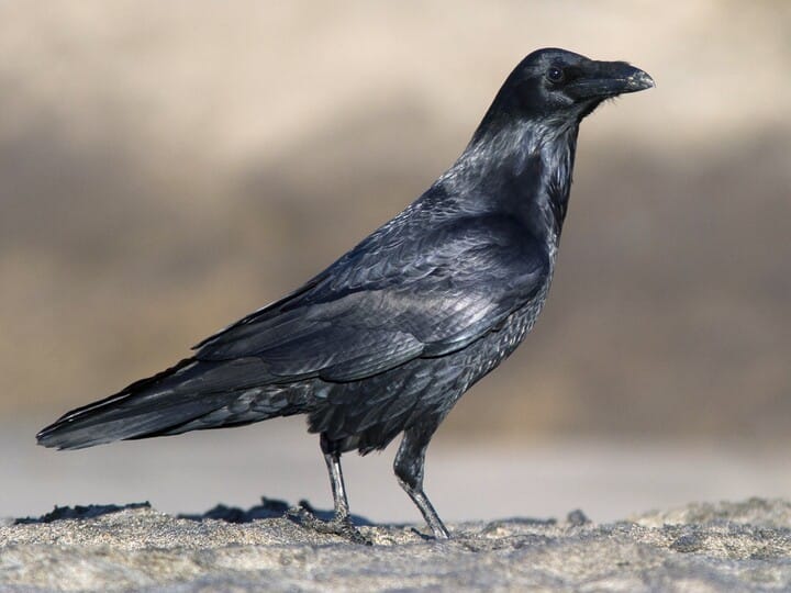
Least Concern	American Crow	15.6	453	4.59	1	30.15	730	730	20	44	Diet data is not available	🌲 Forest 🌿 Grassland 🏖 Coastal 🏙 Urban 🌾 Agricultural 🌊 Estuarine 🌊 Riparian				Common Raven
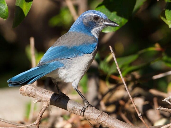
Least Concern	Blue Jay	5.5	85.25	4.34	1	19	365	455.1	26.2	27	Diet data is not available	🌲 Forest				California Scrub-Jay
Least Concern	Trumpeter Swan	214	10,300	5.2	1	98.5	1,095	1,091.94	32.5	158.75	🌿 Plant 🌿 Fern	🌊 Lakes 🌊 Rivers 🌊 Marsh 🌊 Estuarine 🏖 Coastal				Tundra Swan
Least Concern	Tundra Swan	181.25	6,350	4	1	60.25	730	1,001.07	24.1	135	🌿 Plant 🦠 Cyanobacteria	🌊 Lakes 🌊 Rivers 🌊 Marsh 🌊 Estuarine 🏖 Coastal				Trumpeter Swan
Least Concern	Mute Swan	221.5	10,230	5.95	1	135	1,095	1,183.57	70	142.5	Diet data is not available	🌊 Lakes 🌊 Rivers 🌊 Marsh 🏖 Coastal				Tundra Swan
Least Concern	Sooty Grouse	22.6	1,059	7.1	1	10	365	455.1	14	46	Diet data is not available	🌲 Forest ⛰ Mountains				Dusky Grouse
Least Concern	Dusky Grouse	22.6	1,059	7.1	1	10	365	455.1	14	46	Diet data is not available	🌲 Forest ⛰ Mountains				Spruce Grouse
Least Concern	Merlin	13	187.57	4.5	1	30	365	545.2	16	28	🐦 Bird 🐀 Mammal 🦎 Reptile	🏜 Desert 🌿 Grassland 🌲 Chaparral 🌲 Taiga 🏖 Coastal 🌊 Marsh				American Kestrel
Least Concern	Prairie Falcon	30.6	754.5	4.25	1	38.5	365	545.97	20	42	🐦 Bird 🐀 Mammal 🪲 Insect 🦎 Reptile 🕷 Spider 🐸 Amphibian	🏜 Desert 🌿 Grassland 🌲 Chaparral ⛰ Mountains 🌾 Agricultural				Peregrine Falcon
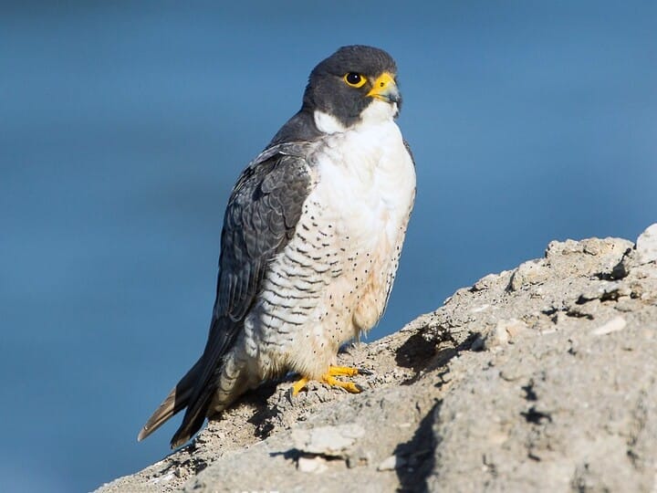
Least Concern	Peregrine Falcon	35.5	827.25	3.5	1	39	365	726.94	25	43	🐦 Bird 🐀 Mammal	🏔 Tundra 🌲 Taiga 🏜 Desert 🌿 Grassland 🌲 Forest ⛰ Mountains 🏙 Urban 🌲 Chaparral				Prairie Falcon
Least Concern	Gyrfalcon	52.08	1,415.75	3.61	1	47.75	730	728.47	13.5	56.5	🐦 Bird 🐀 Mammal	🏔 Tundra				Prairie Falcon
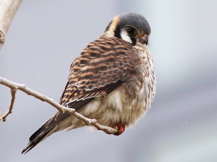
Least Concern	American Kestrel	9	115.5	4.6	1.25	30	365	365	17	24	🐀 Mammal 🪲 Insect 🐦 Bird 🦎 Reptile 🐸 Amphibian 🕷 Spider 🐛 Centipede 🪱 Worm	🏜 Desert 🌿 Grassland 🌲 Chaparral 🌲 Forest ⛰ Mountains 🏙 Urban 🌾 Agricultural				Merlin
Critically Endangered	California Condor	185.3	8,800	1	1	192.5	2,190	2,185.4	45	118	Diet data is not available	🏜 Desert 🌲 Chaparral			Audio is not available	Turkey Vulture
Vulnerable	Pinyon Jay	6.26	105	3.82	1	21	365	545.2	14.58	26.5	🪲 Insect 🌲 Conifer 🕷 Spider 🌿 Plant 🦎 Reptile	🌲 Forest				Mexican Jay
Least Concern	Harlequin Duck	31.45	561.25	5.9	1	40	365	545.97	14.6	44.5	Diet data is not available	🏔 Tundra 🌊 Rivers 🏖 Coastal 🌊 Riparian 🌲 Forest				Long-tailed Duck
Least Concern	Wood Thrush	4.2	48.65	3.5	2	12.25	365	365.12	10.17	20.5	🪲 Insect 🐌 Snail 🕷 Spider	🌲 Forest				Ovenbird
Least Concern	Mississippi Kite	17	281	2	1	34	365	365	11.2	34	🪲 Insect 🐸 Amphibian 🐀 Mammal 🦎 Reptile	🌲 Forest 🌿 Grassland 🌾 Agricultural 🌊 Riparian 🏙 Suburban				White-tailed Kite
Least Concern	Acorn Woodpecker	4.7	79.05	4.9	2	31	766	694	17.25	23	🪲 Insect 🕷 Spider	🌲 Forest 🌳 Rainforest				White-headed Woodpecker
Near Threatened	Black Scoter	44.1	1,052.2	8.5	1	45.75	730	819.34	17.92	48.5	Diet data is not available	🌊 Lakes 🏖 Coastal				Surf Scoter
Least Concern	Wild Turkey	42.25	5,811	11	1	14	365	304	13	85.5	🌿 Plant 🌲 Conifer 🌿 Moss	🌊 Marsh 🌲 Forest 🌾 Agricultural 🌊 Riparian				Ruffed Grouse
Least Concern	Wood Stork	62	2,500	3.02	1	53.75	1,460	1,460	27	95.25	🐟 Fish 🐸 Amphibian 🦀 Crustacean	🌊 Marsh 🌊 Estuarine 🌊 Swamp				White Ibis
Least Concern	Monk Parakeet	4.76	108.63	6	2	42	730	730	22.1	33	Diet data is not available	🌿 Grassland 🌳 Scrub forest				White-winged Parakeet
Least Concern	Clark's Nutcracker	7.1	130	3	1	22	365	365	17.42	31	Diet data is not available	🌲 Forest ⛰ Mountains 🌲 Taiga				Canada Jay
Least Concern	Ruddy Duck	44	550	8	1	55.75	365	365	13.6	38.1	Diet data is not available	🌊 Lakes 🌊 Marsh 🌊 Estuarine 🏖 Coastal				Bufflehead
Least Concern	Indian Peafowl	120	4,093.75	5	1	14	730.25	730	25	95	Diet data is not available	🌿 Grassland 🌲 Forest 🌳 Rainforest 🏙 Urban ⛰ Mountains				Spalding Peafowl
Least Concern	Downy Woodpecker	1.67	27.5	4.8	1.25	21.75	365	365	11.92	16	🪲 Insect 🌿 Plant 🕷 Spider	🌲 Forest ⛰ Mountains 🏙 Urban 🌊 Riparian 🌾 Agricultural			Audio is not available	Hairy Woodpecker
Least Concern	Roseate Spoonbill	50	1,500	3	1	52.5	1,095	1,095	28	75	Diet data is not available	🌊 Marsh				American Flamingo
Least Concern	Glossy Ibis	23.85	633.75	3.5	1	42	1,095	1,095	26.8	52	🪲 Insect 🦀 Crustacean 🦎 Reptile 🕷 Spider 🪱 Worm 🐌 Snail 🐸 Amphibian 🐚 Scallop	🌊 Marsh 🌊 Lakes 🌾 Agricultural 🏖 Coastal				White-faced Ibis
Vulnerable	Steller's Eider	42.5	842	7	1	50	730	819.34	23	45.5	Diet data is not available	🏖 Coastal 🏔 Tundra 🌊 Lakes				Long-tailed Duck
Least Concern	Snail Kite	29.3	382.58	3	1.5	30	365	657.45	17	43.5	Diet data is not available	🌊 Marsh				Hook-billed Kite
Near Threatened	Common Eider	72.7	2,092	4.15	1	58	730	730	37.8	60.5	Diet data is not available	🏔 Tundra 🏖 Coastal				Spectacled Eider
Least Concern	King Eider	42.8	1,650	4.7	1	30	730	819.34	18.92	53	Diet data is not available	🌊 Lakes 🏔 Tundra 🏖 Coastal 🌊 Estuarine				Spectacled Eider
Least Concern	American Robin	5.5	78.78	3.43	2.5	14.3	365	364.23	17	26.5	🪲 Insect 🌿 Plant 🕷 Spider 🌲 Conifer	🌲 Forest 🌳 Scrub forest 🏙 Urban 🌾 Agricultural 🌊 Riparian				Spotted Towhee
1 Life history data from database created by Myhrvold et al. 2015. 2 IUCN data was downloaded from GBIF. 3 Images from valuable contributors to iNaturalist and All About Birds. 4 Diet data download from R package {aviandietdb}. 5 Birds habitat data collected from Animal Biodiversity Web and All About Birds. 6 Data gathered from USGS Breeding Bird Survey. 7 Range data with 9km resolution downloaded from eBird. 8 Bird call data was collected from Xeno-canto and downloaded from GBIF.

Things I couldn’t get work

There are a couple of features that I tried to implement but couldn’t get them work. For example, I couldn’t customize column widths with gt::cols_width function. I also was not able to use gt::opt_interactive to add filtering, sorting, searching, pagination features to the table. Any advice on how to make them work would be greatly appreciated 🥰!

Acknowledgement

All the wonderful photographers that shared their bird photos on iNaturalist and All About Birds 💗.

GitHub Copilot in R Studio: contributions to document narrative, code completion and comments.

ChatGPT: contributions to data transformation, emoji suggestions, filling in domain knowledge gap, and code help.

References

Hurlbert, AH, AM Olsen, MM Sawyer, and PM Winner. 2021. The Avian Diet Database as a quantitative source of information on avian diets. Scientific Data 8:260. https://doi.org/10.1038/s41597-021-01049-9

IUCN (2022). The IUCN Red List of Threatened Species. Version 2022-2. https://www.iucnredlist.org. Downloaded on 2023-05-09. https://doi.org/10.15468/0qnb58 accessed via GBIF.org on 2023-11-17. accessed via GBIF.org on 2024-05-17.

Matthew Strimas-Mackey, Shawn Ligocki, Tom Auer, Daniel Fink (2023). ebirdst: Access and Analyze eBird Status and Trends Data Products. R package version 3.2022.0. https://ebird.github.io/ebirdst/

Myhrvold, N.P., Baldridge, E., Chan, B., Sivam, D., Freeman, D.L., Ernest, S.K.M., 2015. An amniote life-history database to perform comparative analyses with birds, mammals, and reptiles. Ecology 96, 3109–3109. https://doi.org/10.1890/15-0846R.1

Vellinga W (2024). Xeno-canto - Bird sounds from around the world. Xeno-canto Foundation for Nature Sounds. Occurrence dataset https://doi.org/10.15468/qv0ksn accessed via GBIF.org on 2024-05-23.

Ziolkowski, D.J., Lutmerding, M., English, W.B., Aponte, V.I., and Hudson, M-A.R., 2023, North American Breeding Bird Survey Dataset 1966 - 2022: U.S. Geological Survey data release, https://doi.org/10.5066/P9GS9K64.